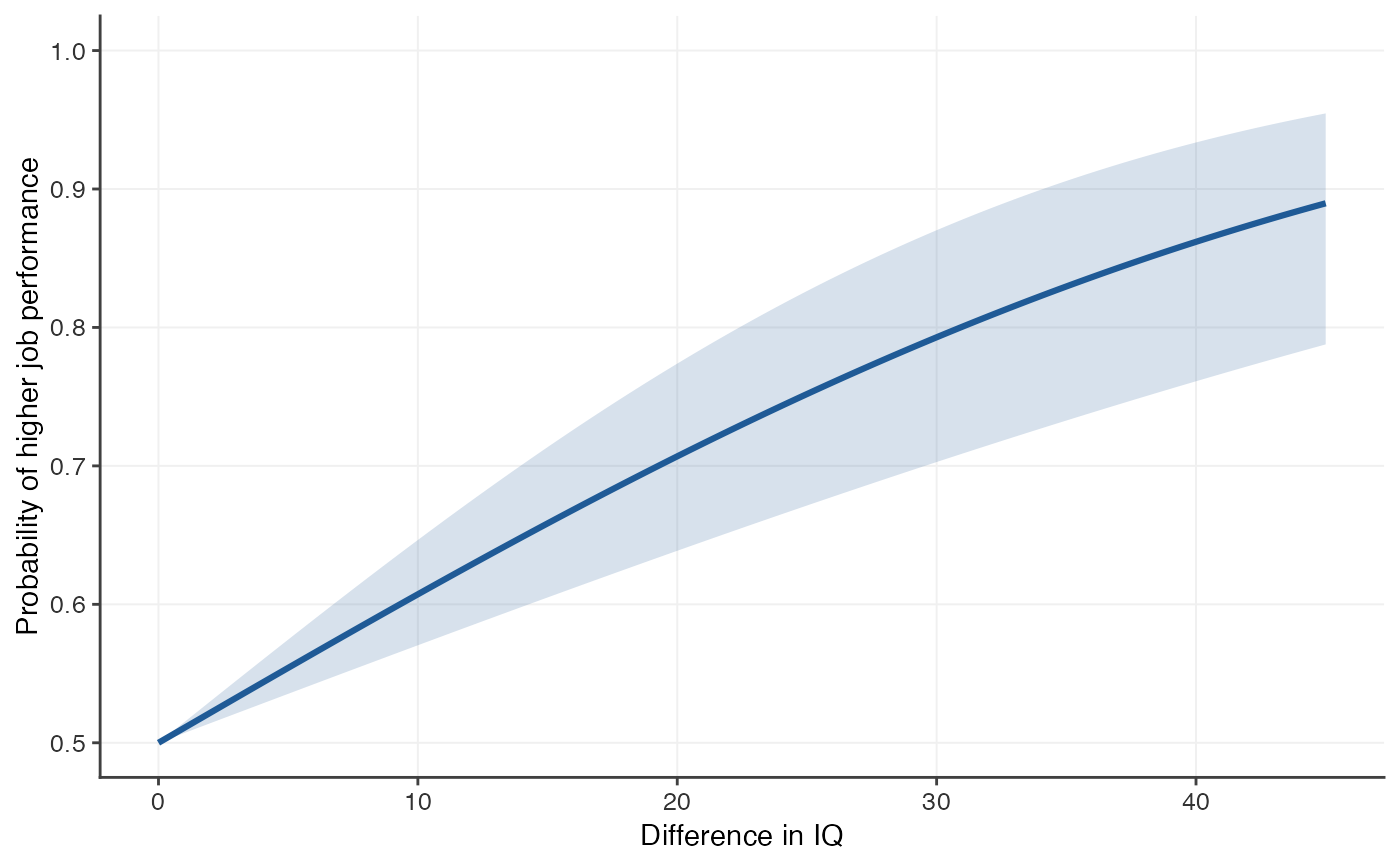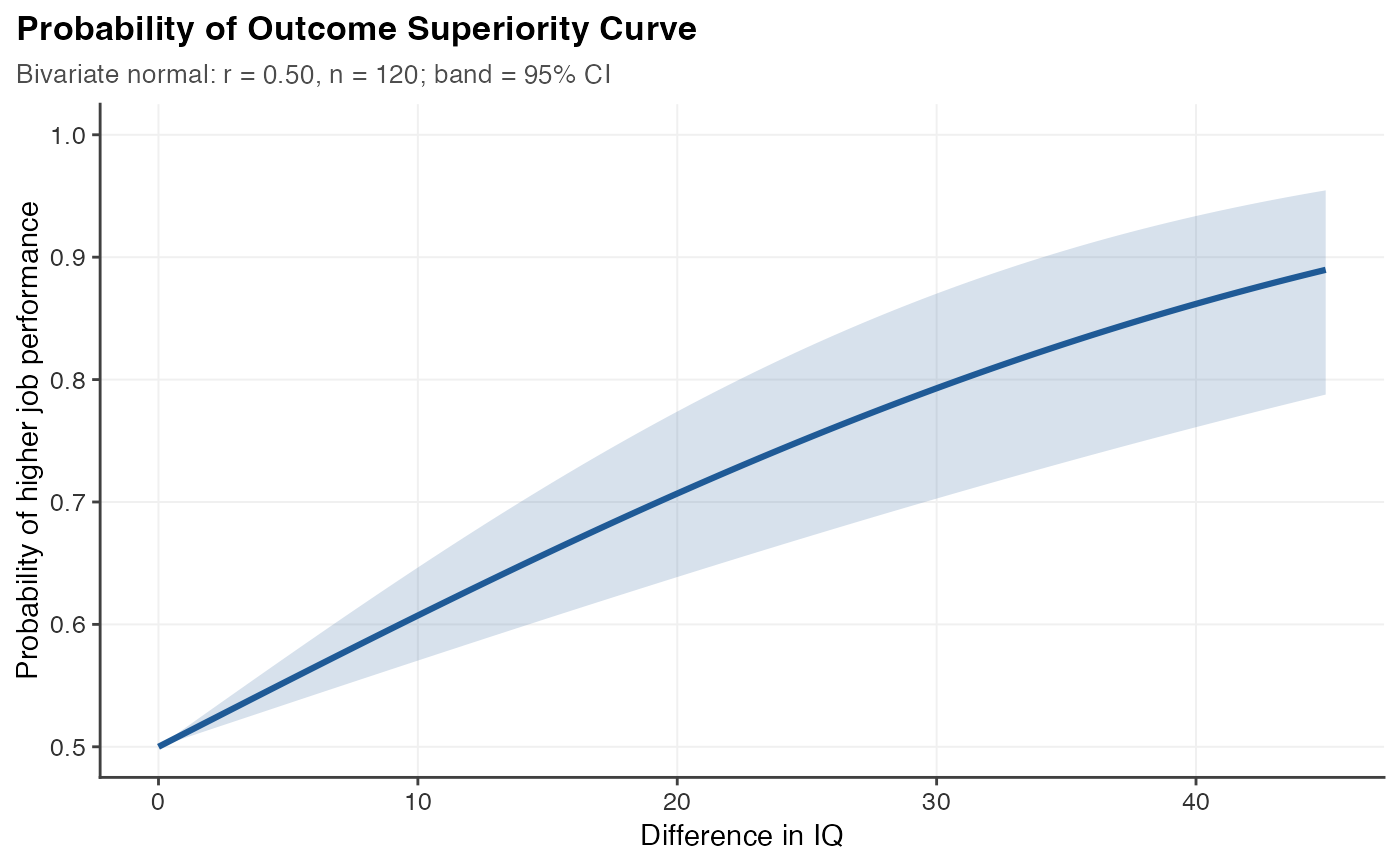
autoplot() returns a ggplot2::ggplot() object that can be modified
further; plot() draws it.
Arguments
- object, x
A
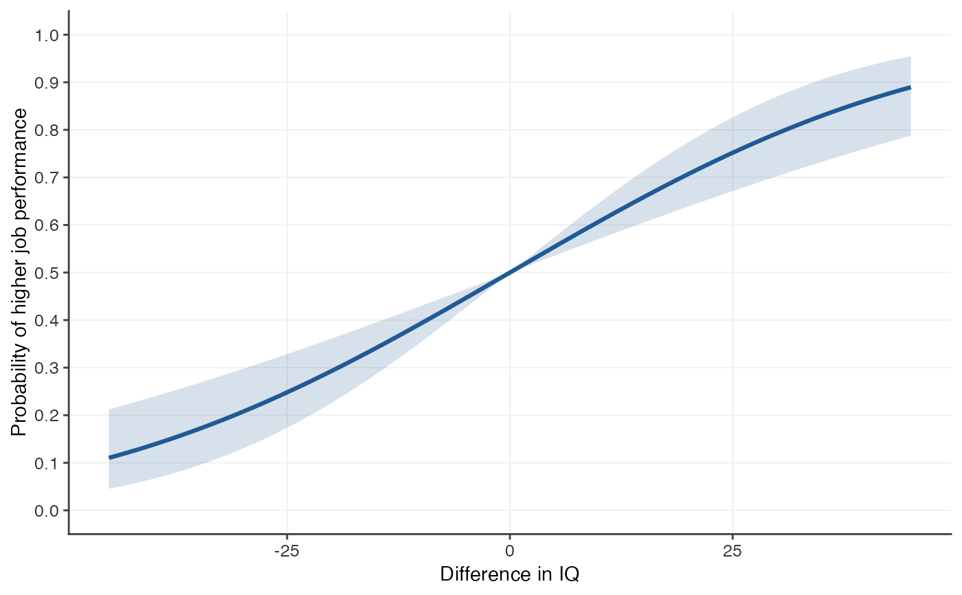
"posc"object.- full
If
FALSE(default), plot differences \(\Delta \ge 0\), where the curve runs from 0.5 upwards (or downwards for a negative relationship). IfTRUE, plot the full sigmoid over negative and positive differences. The two halves are mirror images, since \(P(-\Delta) = 1 - P(\Delta)\).- color
Colour of the curve and its confidence band.
- ci
Draw the confidence band (if one is available)?
- reference
For empirical curves from
posc_emp(): also draw the bivariate-normal POSC with the same Pearson correlation, as a dashed line? Off by default.- bins
For empirical curves fitted with bins: draw the binned observed proportions as points, with whiskers showing simultaneous confidence intervals (see
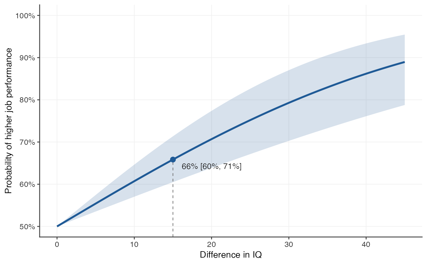
posc_bins())? Off by default.- percent
Label the probability axis as percentages (50, 60, ...) instead of probabilities (0.5, 0.6, ...)?
- grid
Draw light gridlines?
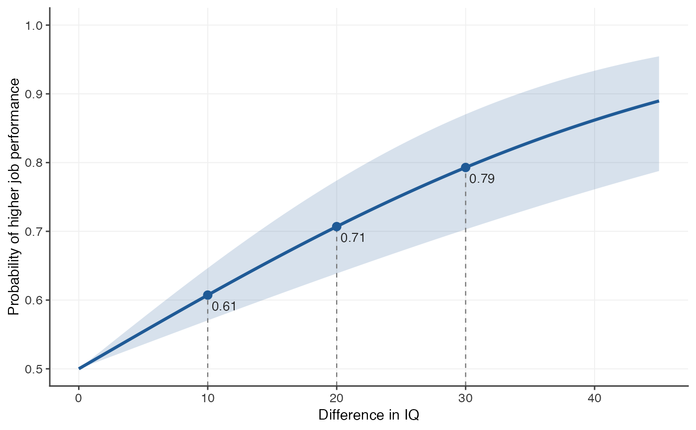
- mark
Optional numeric vector of differences in the predictor to highlight. For each one, a guide line runs up from the x-axis to the curve and the probability is labelled at the point. Negative values are only shown when
full = TRUE.- mark_ci
Add the confidence interval to the labels of marked points?
- title, subtitle
Plot title and subtitle. None by default; supply a string, or
TRUEfor an automatic one (the subtitle then describes the method, correlation, sample size and band).- ...
Passed from
plot()toautoplot().
Value
autoplot() returns a ggplot object; plot() returns it
invisibly.