Empirical POSC from raw data

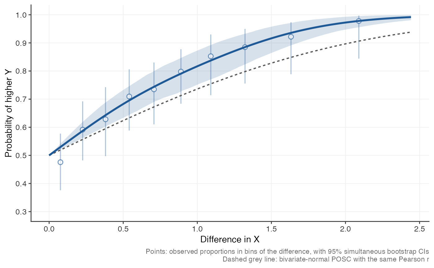
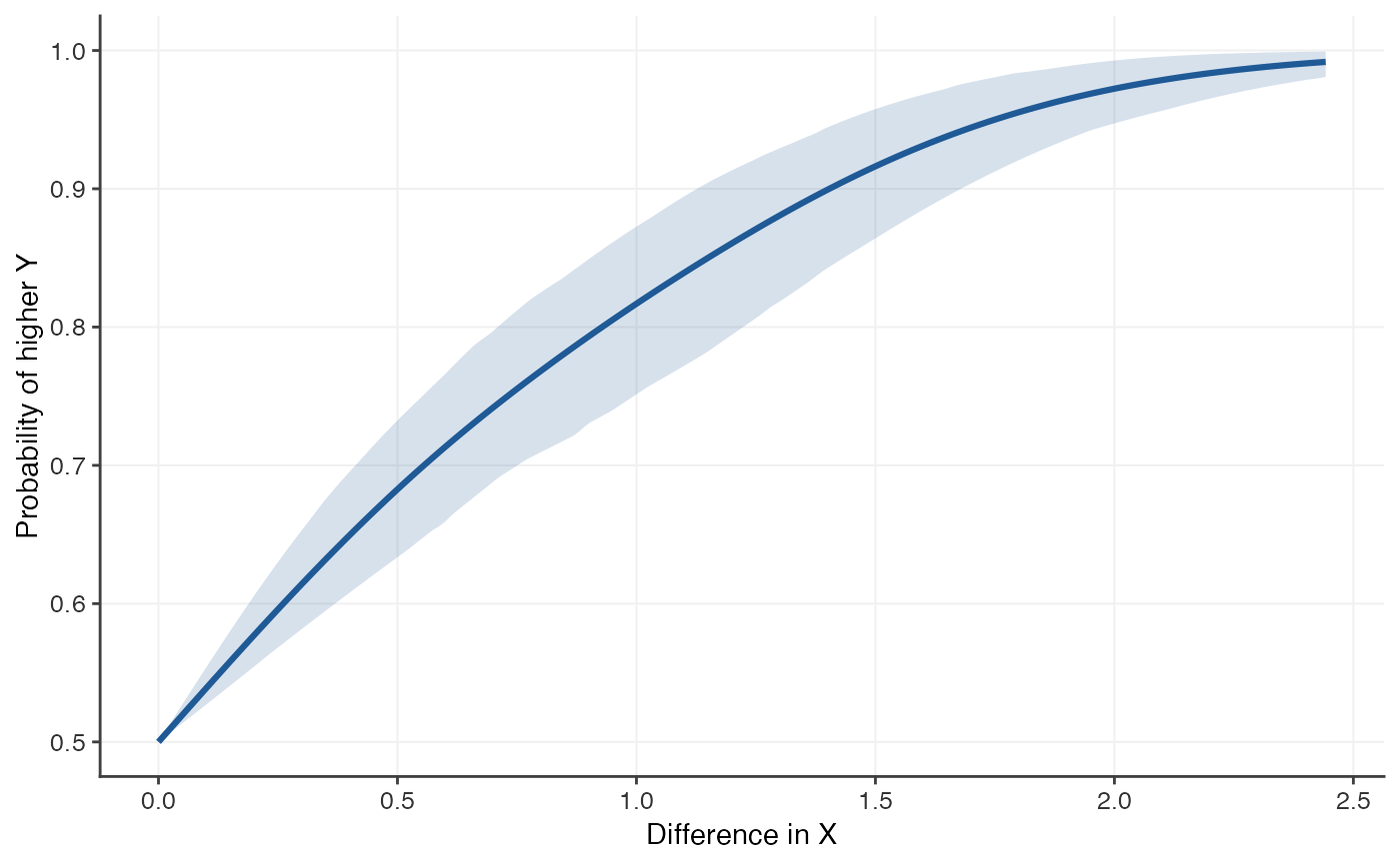
Estimates the probability of outcome superiority curve directly from predictor and outcome scores, without assuming bivariate normality, with a bootstrap confidence band.

Usage

posc_emp(
  x,
  y,
  df = 3,
  level = 0.95,
  n_boot = 1000,
  max_pairs = 20000,
  max_delta = NULL,
  bins = 10,
  standardize = FALSE,
  predictor_name = "X",
  outcome_name = "Y"
)

Arguments

x, y: Numeric vectors of predictor and outcome scores. Pairs with a missing value in either are dropped.
df: Degrees of freedom of the spline (1 to 10).
level: Confidence level of the band.
n_boot: Number of bootstrap resamples. At least 1000 is recommended for a 95 percent band; use 0 for no band.
max_pairs: Maximum number of pairs used in each fit.
max_delta: Largest difference in the predictor to evaluate. Defaults to the 95th percentile of the absolute pairwise differences.
bins: Bins for the observed proportions: either the number of bins (default 10), which are formed to hold roughly equal numbers of pairs, or a vector of breakpoints for $|\Delta|$ (in the units of the predictor, after standardizing if standardize = TRUE). Use 0 or NULL for no bins.
standardize: If TRUE, the predictor is standardized first so that differences are in standard-deviation units.
predictor_name, outcome_name: Labels used in printed output and plots.

Value

An object of class "posc": a list with elements

curve: data frame with columns delta, p, lower, upper, over a symmetric grid of differences.
method, r, n, level, sd_x, max_delta, labels, details: information about how the curve was computed.

Use plot(), summary() and predict() to work with it.

Details

Pairwise data. Every pair of people $(i, j)$ with $x_i \ne x_j$ contributes the difference $\Delta_{ij} = x_i - x_j$ and an indicator of whether the person with the higher predictor score also has the higher outcome (ties in the outcome count as 1/2). For large samples a random subset of max_pairs pairs is used.

Model. The curve is modelled as $$\mathrm{logit}\, P(\Delta) = \mathrm{sign}(\Delta)\, g(|\Delta|),$$ where $g$ is a natural cubic spline with df degrees of freedom and no intercept, whose basis is zero at $|\Delta| = 0$. This builds in the two properties every POSC must have, $P(0) = 0.5$ and $P(-\Delta) = 1 - P(\Delta)$, while leaving the shape free. The 0/1 responses are shrunk by 0.0005 towards 0.5 so that the fit exists even for near-perfect relationships; this changes the curve by a negligible amount. Increase df for a more flexible curve; df = 1 makes the logit of the curve linear in $\Delta$. Because a natural spline has zero curvature at its boundary, the curve is smooth through $\Delta = 0$. It is not forced to be monotone.

Confidence band. Pairs that share a person are not independent, so model-based standard errors from the pairwise regression would be far too small. Instead, people are resampled with replacement n_boot times, the curve is refitted to each resample (with the knots held fixed), and the band is formed from pointwise percentiles of the bootstrap curves. Pairs formed by a person and their own duplicate are excluded. Use set.seed() beforehand for reproducible results.

Binned observed proportions. To check the fitted curve against the data, the pairs with $|\Delta| \le$ max_delta are grouped into bins of $|\Delta|$ and the observed proportion of pairs in which the person higher on the predictor is also higher on the outcome is computed in each bin. plot(fit, bins = TRUE) shows these as points with whiskers, and posc_bins() returns them as a table. The whiskers are simultaneous (family-wise) confidence intervals: with probability level they cover all of the bin proportions at once. They are computed from the same person-level bootstrap as the curve, on the empirical-logit scale $\ell_k = \mathrm{logit}\{(n_k \hat p_k + 0.5)/(n_k + 1)\}$ for a bin with $n_k$ pairs: the interval is $\mathrm{logit}^{-1}(\ell_k \pm c\,\widehat{se}_k)$, where $\widehat{se}_k$ is the bootstrap standard error of $\ell_k$ and $c$ is the level quantile of $\max_k |\ell^*_k - \ell_k| / \widehat{se}_k$ over the bootstrap resamples (the max-$t$ or sup-$t$ method). The intervals are therefore asymmetric and lie between 0 and 1.

Non-monotone relationships. A POSC averages over where in the predictor's distribution a pair of people sits. For a U-shaped relationship, the person higher on the predictor is more likely to have the higher outcome on one side of the minimum and less likely on the other, so the curve reflects the balance of the two. For a symmetric U centred on the middle of the predictor's distribution the true POSC is flat at 0.5, even though the predictor is strongly related to the outcome. The empirical curve is not constrained to be monotone and recovers such shapes; the dashed normal-theory reference, which depends only on the linear correlation, is not meaningful in that case.

Examples

set.seed(1)
x <- rnorm(120)
y <- exp(0.8 * x + rnorm(120, sd = 0.6))   # skewed, non-normal outcome

fit <- posc_emp(x, y, n_boot = 200)   # use n_boot >= 1000 in practice
fit
#> Probability of Outcome Superiority Curve
#>   Method:    empirical (spline logistic, bootstrap CI)
#>   Predictor: X    Outcome: Y
#>   r = 0.618 (Pearson), n = 120
#>   Spline df = 3, pairs used = 7140, bootstrap resamples = 200
#> 
#>   P(higher Y | X higher by delta):
#>  delta     p lower upper
#>  0.441 0.663 0.619 0.711
#>  0.882 0.789 0.725 0.844
#>  1.763 0.951 0.915 0.982
plot(fit)

posc_bins(fit)
#>    delta_low delta_high      delta n_pairs         p     lower     upper
#> 1  0.0000000  0.1518521 0.07622528     679 0.4756996 0.3760137 0.5774302
#> 2  0.1518521  0.3050298 0.22624334     678 0.5914454 0.4821749 0.6921316
#> 3  0.3050298  0.4574587 0.38062235     678 0.6283186 0.4972460 0.7425794
#> 4  0.4574587  0.6206429 0.54051079     678 0.7094395 0.5885122 0.8060455
#> 5  0.6206429  0.7950737 0.70750015     679 0.7349043 0.6102759 0.8302333
#> 6  0.7950737  0.9880430 0.88952408     678 0.7979351 0.6838202 0.8776170
#> 7  0.9880430  1.2004087 1.09102549     678 0.8525074 0.7139100 0.9299624
#> 8  1.2004087  1.4614854 1.32207878     678 0.8849558 0.7555483 0.9498317
#> 9  1.4614854  1.8222753 1.63233955     678 0.9218289 0.7883631 0.9734716
#> 10 1.8222753  2.4420696 2.09021785     679 0.9779087 0.8442007 0.9970605
plot(fit, bins = TRUE, reference = TRUE)   # add data and normal curve

Usage

Arguments

Value

Details

See also

Examples