POSC from a single correlation (bivariate normal)

Computes the probability of outcome superiority curve implied by a correlation between a predictor and an outcome, assuming the two are bivariate normal.

Usage

posc_uni(
  r,
  n = NULL,
  sd_x = 1,
  level = 0.95,
  max_delta = 3 * sd_x,
  predictor_name = "X",
  outcome_name = "Y"
)

Arguments

r

Correlation between predictor and outcome, in \((-1, 1)\).

n

Sample size used to estimate r. Needed for the confidence band; use NULL to draw the curve without one.

sd_x

Standard deviation of the predictor. The curve is expressed in the predictor's units; the default 1 gives standard-deviation units.

level

Confidence level of the band.

max_delta

Largest difference in the predictor to evaluate. Defaults to 3 standard deviations of the predictor.

predictor_name, outcome_name

Labels used in printed output and plots.

Value

An object of class "posc": a list with elements

curve

data frame with columns delta, p, lower, upper, over a symmetric grid of differences.

method, r, n, level, sd_x, max_delta, labels, details

information about how the curve was computed.

Use plot(), summary() and predict() to work with it.

Details

If \(X\) and \(Y\) are bivariate normal with correlation \(r\), then for two randomly chosen people whose predictor scores differ by \(\Delta\) $$P(Y_1 > Y_2 \mid X_1 - X_2 = \Delta) = \Phi\left(\frac{r\,\Delta / \sigma_X}{\sqrt{2(1 - r^2)}}\right),$$ where \(\Phi\) is the standard normal distribution function and \(\sigma_X\) the standard deviation of the predictor. Set sd_x to put \(\Delta\) on the raw scale of the predictor; the default sd_x = 1 gives differences in standard-deviation units.

The curve is monotone in \(r\), so the pointwise confidence band is obtained by evaluating it at the limits of the Fisher-\(z\) confidence interval for \(r\).

See also

posc_emp() for a curve estimated from raw data without assuming normality; posc_comp() to compare curves.

Examples

# Differences in SD units
fit <- posc_uni(r = 0.5, n = 100)
fit
#> Probability of Outcome Superiority Curve
#>   Method:    bivariate normal
#>   Predictor: X    Outcome: Y
#>   r = 0.500, 95% CI [0.337, 0.634], n = 100
#> 
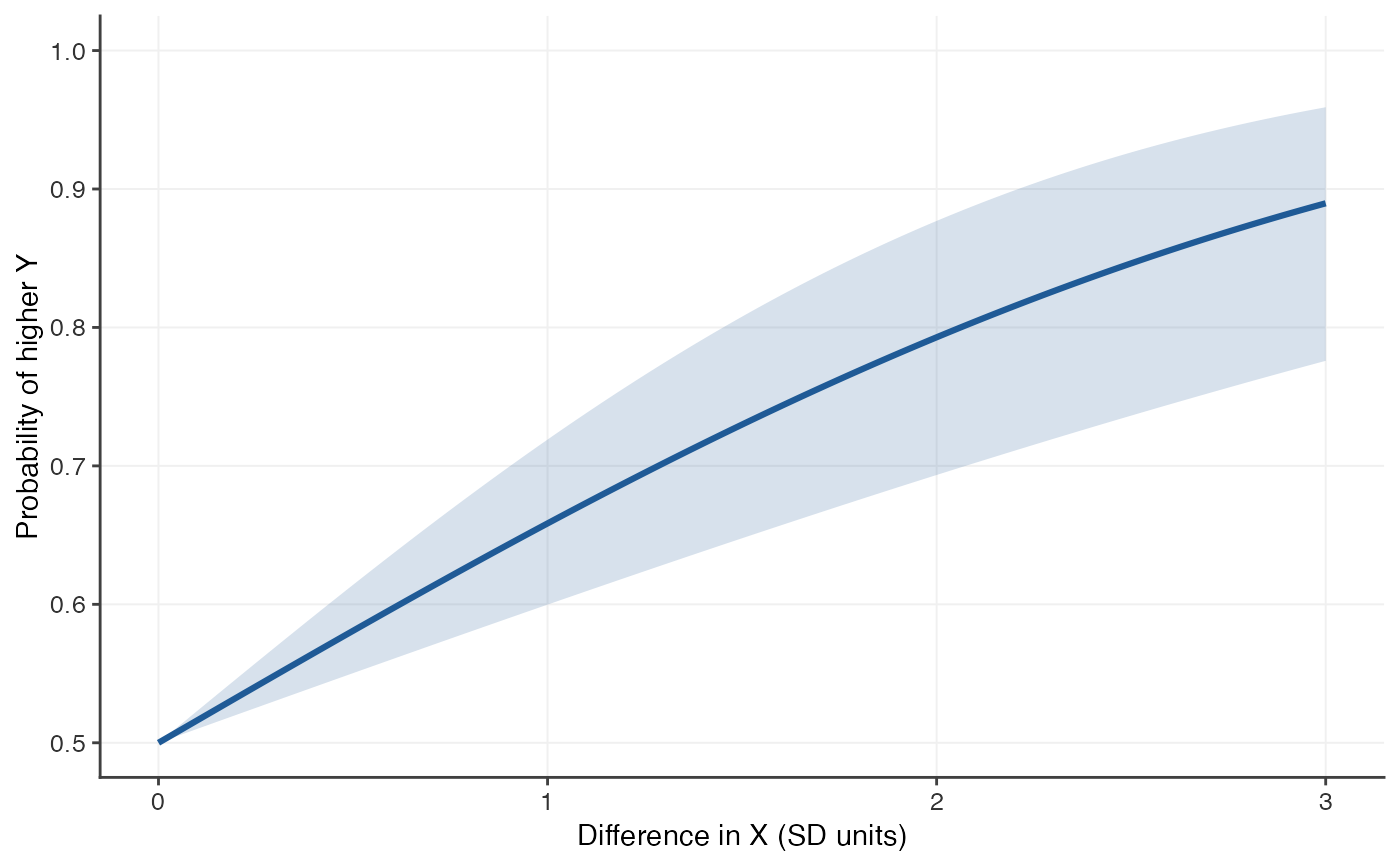
#>   P(higher Y | X higher by delta):
#>  delta     p lower upper
#>  0.500 0.581 0.550 0.614
#>  1.000 0.658 0.600 0.719
#>  2.000 0.793 0.693 0.877
plot(fit)


# Raw units: an IQ test with SD = 15
iq <- posc_uni(r = 0.5, n = 100, sd_x = 15, predictor_name = "IQ",
               outcome_name = "job performance")
predict(iq, delta = c(5, 15, 30))
#>   delta         p     lower     upper
#> 1     5 0.5541221 0.5335775 0.5766406
#> 2    15 0.6584543 0.5997878 0.7190156
#> 3    30 0.7928919 0.6934299 0.8769429