Compare probability of outcome superiority curves

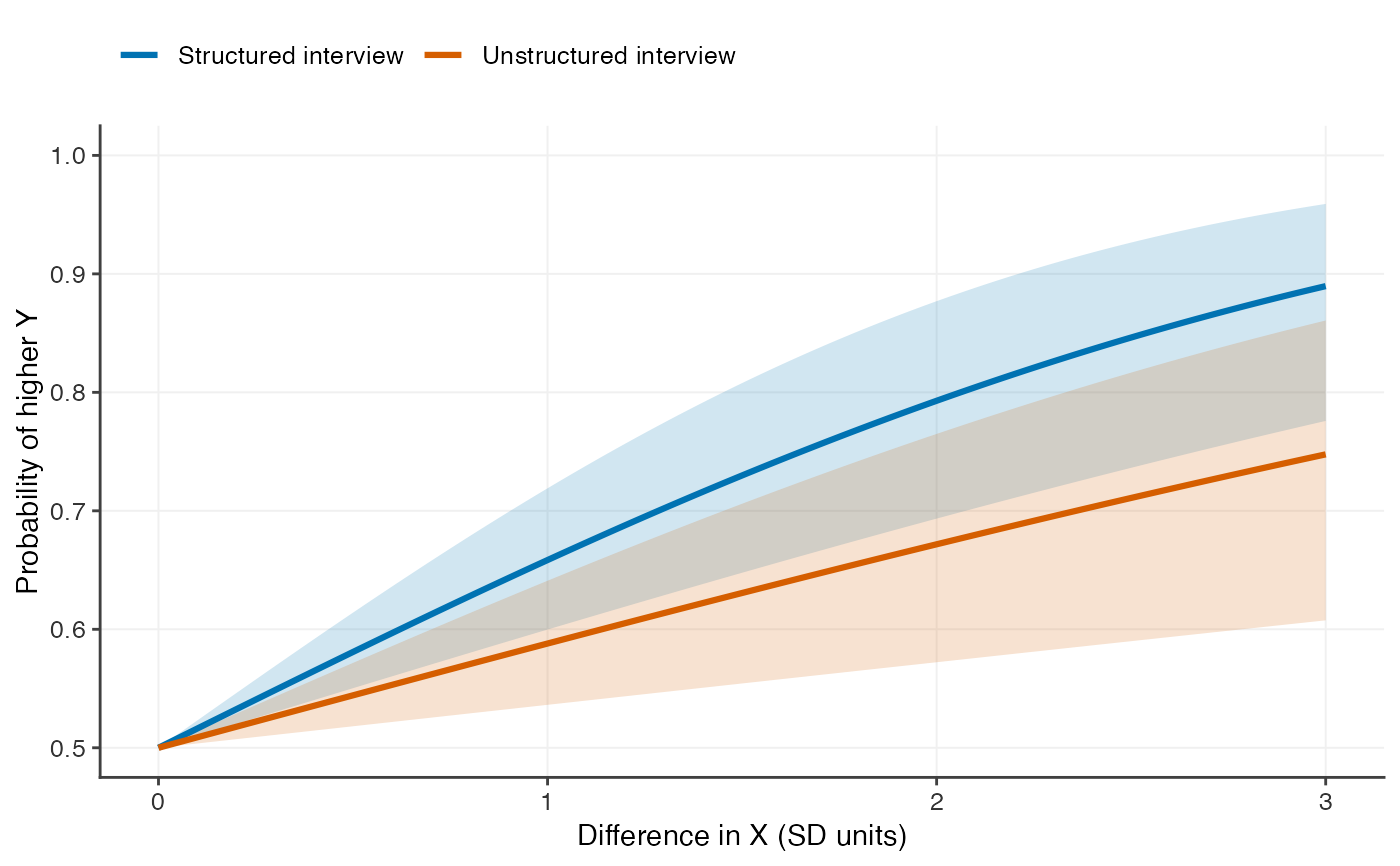
Overlays several POSCs and tests whether their underlying correlations differ.

Usage

posc_comp(..., labels = NULL)

Arguments

...

Two or more "posc" objects, optionally named (the names are used as labels). A single list of "posc" objects is also accepted.

labels

Optional character vector of labels, one per curve.

Value

An object of class "posc_comparison", a list with elements posc (the curves), table (a data frame of each curve's method, correlation and sample size) and test (a list with the statistic, degrees of freedom and p-value, or NULL). It has print(), plot() and ggplot2::autoplot() methods.

Details

Under bivariate normality a POSC is determined entirely by its correlation, so curves from independent samples can be compared by testing whether the correlations are equal. For two curves this is the usual Fisher-\(z\) test, $$z = \frac{\tanh^{-1} r_1 - \tanh^{-1} r_2} {\sqrt{1/(n_1 - 3) + 1/(n_2 - 3)}};$$ for more than two it is the homogeneity test \(Q = \sum_i (n_i - 3)(z_i - \bar z)^2\), referred to a \(\chi^2\) distribution with one fewer degrees of freedom than curves, where \(\bar z\) is the weighted mean of the \(z_i\).

Both tests assume the curves come from independent samples. For curves from posc_emp() the test compares the Pearson correlations, not the shapes of the curves. No test is reported if any curve lacks a sample size.

Examples

a <- posc_uni(r = 0.5, n = 100)
b <- posc_uni(r = 0.3, n = 120)
cmp <- posc_comp(`Structured interview` = a, `Unstructured interview` = b)
cmp
#> Comparison of 2 probability of outcome superiority curves
#> 
#>  curve                  method r     n  
#>  Structured interview   normal 0.500 100
#>  Unstructured interview normal 0.300 120
#> 
#> Test of equal correlations (independent samples):
#>   z = 1.75, p = 0.0808
plot(cmp)